Blade Mesher
The PGL.components.blademesher.BladeMesher generates a 3D surface mesh around a rotor, combining the classes for blade surface, root or nacelle, and blade tip.
There are two examples that generate a mesh around a rotor; one with a simple cylindrical root connection, and another with a full spinner and nacelle geoemtry.
BladeMesher Simple Root Example
In this example, we will generate a mesh around the three bladed DTU 10MW RWT with a simple cylindrical root connection.
The example is located in PGL/examples/blademesher_example.py.
import numpy as np

from PGL.main.blademesher import BladeMesher
from PGL.main.planform import read_blade_planform
from PGL.main.domain import write_x2d

m = BladeMesher()

# path to the planform
m.planform_filename = 'data/DTU_10MW_RWT_blade_axis_prebend.dat'

# spanwise and chordwise number of vertices
m.ni_span = 129
m.ni_chord = 257

# redistribute points chordwise
m.redistribute_flag = True
# number of points on blunt TE
m.chord_nte = 9
# set min TE thickness (which will open TE using AirfoilShape.open_trailing_edge)
# d.minTE = 0.0002

# user defined cell size at LE
# when left empty, ds will be determined based on
# LE curvature
# m.dist_LE = np.array([])

# airfoil family - can also be supplied directly as arrays
m.blend_var = [0.241, 0.301, 0.36, 0.48, 1.0]
m.base_airfoils_path = ['data/ffaw3241.dat',
                        'data/ffaw3301.dat',
                        'data/ffaw3360.dat',
                        'data/ffaw3480.dat',
                        'data/cylinder.dat']

# number of vertices and cell sizes in root region
m.root_type = 'cylinder'
m.ni_root = 8
m.s_root_start = 0.0
m.s_root_end = 0.065
m.ds_root_start = 0.008
m.ds_root_end = 0.005

# add additional dist points to e.g. refine the root
# for placing VGs
# self.pf_spline.add_dist_point(s, ds, index)

# inputs to the tip component
# note that most of these don't need to be changed
m.ni_tip = 11
m.s_tip_start = 0.99
m.s_tip = 0.995
m.ds_tip_start = 0.001
m.ds_tip = 0.00005

m.tip_fLE1 = .5  # Leading edge connector control in spanwise direction.
                 # pointy tip 0 <= fLE1 => 1 square tip.
m.tip_fLE2 = .5  # Leading edge connector control in chordwise direction.
                 # pointy tip 0 <= fLE1 => 1 square tip.
m.tip_fTE1 = .5  # Trailing edge connector control in spanwise direction.
                 # pointy tip 0 <= fLE1 => 1 square tip.
m.tip_fTE2 = .5  # Trailing edge connector control in chordwise direction.
                 # pointy tip 0 <= fLE1 => 1 square tip.
m.tip_fM1 = 1.   # Control of connector from mid-surface to tip.
                 # straight line 0 <= fM1 => orthogonal to starting point.
m.tip_fM2 = 1.   # Control of connector from mid-surface to tip.
                 # straight line 0 <= fM2 => orthogonal to end point.
m.tip_fM3 = .2   # Controls thickness of tip.
                 # 'Zero thickness 0 <= fM3 => 1 same thick as tip airfoil.

m.tip_dist_cLE = 0.0001  # Cell size at tip leading edge starting point.
m.tip_dist_cTE = 0.0001  # Cell size at tip trailing edge starting point.
m.tip_dist_tip = 0.00025  # Cell size of LE and TE connectors at tip.
m.tip_dist_mid0 = 0.00025  # Cell size of mid chord connector start.
m.tip_dist_mid1 = 0.00004  # Cell size of mid chord connector at tip.

m.tip_c0_angle = 40.  # Angle of connector from mid chord to LE/TE

m.tip_nj_LE = 20   # Index along mid-airfoil connector used as starting point for tip connector


# generate the mesh
m.update()

# rotate domain with flow direction in the z+ direction and blade1 in y+ direction
m.domain.rotate_x(-90)
m.domain.rotate_y(180)

# copy blade 1 to blade 2 and 3 and rotate
m.domain.add_group('blade1', list(m.domain.blocks.keys()))
m.domain.rotate_z(-120, groups=['blade1'], copy=True)
m.domain.rotate_z(120, groups=['blade1'], copy=True)

# We scale back to real size with the total radius
m.domain.scale(89.166)

# split blocks to cubes of size 33^3
m.domain.split_blocks(33)

# Write EllipSys3D ready surface mesh
write_x2d(m.domain)
# Write Plot3D surface mesh (in real size, not PGL normalization)
m.domain.write_plot3d('DTU_10MW_RWT_mesh.xyz')
BladeMesher With Nacelle Example
To build the rotor mesh including a spinner and nacelle, you need to supply a few extra inputs.
The example in PGL/examples/blademesher_nacelle_example.py shows how to add a spinner/nacelle, replacing the simple cylindrical root from the above example.
import numpy as np

from PGL.main.blademesher import BladeMesher
from PGL.main.planform import read_blade_planform
from PGL.main.bezier import BezierCurve
from PGL.main.curve import SegmentedCurve, Curve
from PGL.main.domain import write_x2d

m = BladeMesher()

# path to the planform
m.planform_filename = 'data/DTU_10MW_RWT_blade_axis_prebend.dat'

# spanwise and chordwise number of vertices
m.ni_span = 129
m.ni_chord = 257

# redistribute points chordwise
m.redistribute_flag = True
# number of points on blunt TE
m.chord_nte = 9
# set min TE thickness (which will open TE using AirfoilShape.open_trailing_edge)
# d.minTE = 0.0002

# user defined cell size at LE
# when left empty, ds will be determined based on
# LE curvature
# m.dist_LE = np.array([])

# airfoil family - can also be supplied directly as arrays
m.blend_var = [0.241, 0.301, 0.36, 0.48, 1.0]
m.base_airfoils_path = ['data/ffaw3241.dat',
                        'data/ffaw3301.dat',
                        'data/ffaw3360.dat',
                        'data/ffaw3480.dat',
                        'data/cylinder.dat']


# tell the mesher to add a nacelle object and generate a nacelle shape
m.root_type = 'nacelle'

c = BezierCurve()
CPs = np.array([[-6.5, 0],
                [-6.5, 1.5],
                [-4., 2.86],
                [-2.0, 3.],
                [-0.5, 3.25],
                [3.5, 3.5]])
CPs[:,1] *= 4./3.5
CPs /= 89.166
c.CPs = CPs
c.update()
c1 = Curve(points=np.array([np.linspace(3.5,18.5,100),np.linspace(4.,4.,100)]).T)
c1.points /= 89.166
sc = SegmentedCurve()
sc.add_segment(c)
sc.add_segment(c1)
sc.update()

m.nacelle_curve = sc
m.blade_root_radius = 5.38 / 2 / 89.166
m.hub_length = 6.5/ 89.166
m.dr_junction = 0.075
m.ni_root = 16
m.s_root_end = 0.065
m.ds_root_start = 0.001
m.ds_root_end = 0.005
m.base_nv = 7
m.ds_base = 0.0005
m.nacelle_dr = 0.5/89.166
m.ds_nacelle = 0.0012

# add additional dist points to e.g. refine the root
# for placing VGs
# self.pf_spline.add_dist_point(s, ds, index)

# inputs to the tip component
# note that most of these don't need to be changed
m.ni_tip = 11
m.s_tip_start = 0.99
m.s_tip = 0.995
m.ds_tip_start = 0.001
m.ds_tip = 0.00005

m.tip_fLE1 = .5  # Leading edge connector control in spanwise direction.
                 # pointy tip 0 <= fLE1 => 1 square tip.
m.tip_fLE2 = .5  # Leading edge connector control in chordwise direction.
                 # pointy tip 0 <= fLE1 => 1 square tip.
m.tip_fTE1 = .5  # Trailing edge connector control in spanwise direction.
                 # pointy tip 0 <= fLE1 => 1 square tip.
m.tip_fTE2 = .5  # Trailing edge connector control in chordwise direction.
                 # pointy tip 0 <= fLE1 => 1 square tip.
m.tip_fM1 = 1.   # Control of connector from mid-surface to tip.
                 # straight line 0 <= fM1 => orthogonal to starting point.
m.tip_fM2 = 1.   # Control of connector from mid-surface to tip.
                 # straight line 0 <= fM2 => orthogonal to end point.
m.tip_fM3 = .2   # Controls thickness of tip.
                 # 'Zero thickness 0 <= fM3 => 1 same thick as tip airfoil.

m.tip_dist_cLE = 0.0001  # Cell size at tip leading edge starting point.
m.tip_dist_cTE = 0.0001  # Cell size at tip trailing edge starting point.
m.tip_dist_tip = 0.00025  # Cell size of LE and TE connectors at tip.
m.tip_dist_mid0 = 0.00025  # Cell size of mid chord connector start.
m.tip_dist_mid1 = 0.00004  # Cell size of mid chord connector at tip.

m.tip_c0_angle = 40.  # Angle of connector from mid chord to LE/TE

m.tip_nj_LE = 20   # Index along mid-airfoil connector used as starting point for tip connector


# generate the mesh
m.update()

# rotate domain with flow direction in the z+ direction and blade1 in y+ direction
m.domain.rotate_x(-90)
m.domain.rotate_y(180)

# copy blade 1 to blade 2 and 3 and rotate
m.domain.add_group('blade1', list(m.domain.blocks.keys()))
m.domain.rotate_z(-120, groups=['blade1'], copy=True)
m.domain.rotate_z(120, groups=['blade1'], copy=True)

# We scale back to real size with the total radius
m.domain.scale(89.166)

# split blocks to cubes of size 33^3
m.domain.split_blocks(33)

# Write EllipSys3D ready surface mesh
write_x2d(m.domain)
# Write Plot3D surface mesh
m.domain.write_plot3d('DTU_10MW_RWT_nacelle_mesh.xyz')
The nacelle curve is in this example generated manually from a composite curve consisting of a Bezier curve and a straight line. Note that since the nacelle and spinner will be generated as a rotationally symmetric shape, the curve has to describe only the half the geometry, and should be open ended.
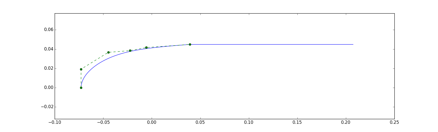
Instead of generating the nacelle shape manually, you can load in the shape from a file.
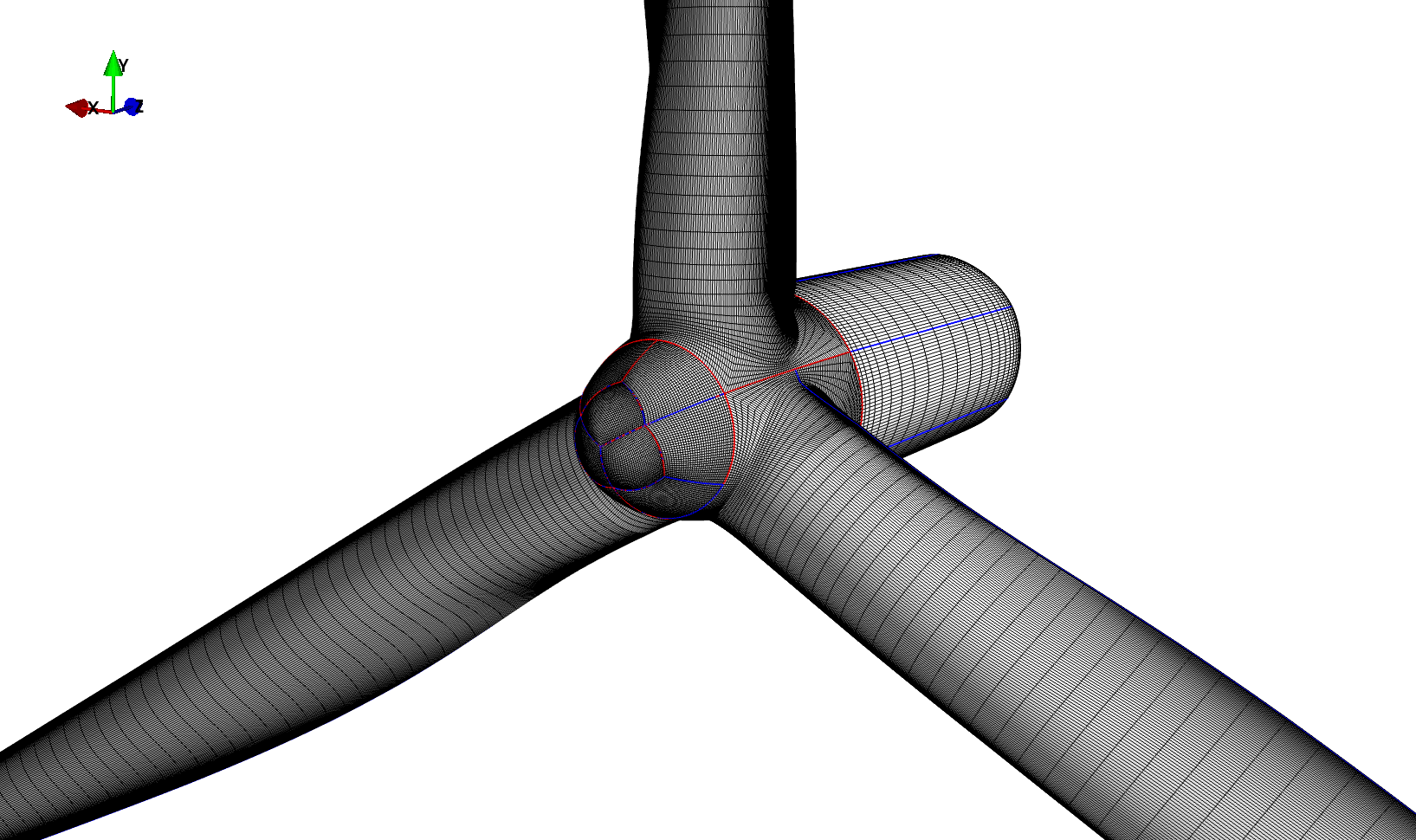
The resulting mesh should look like this:
BladeMesher One Bladed Example
In this example, we will generate a mesh around a single blade which requires the use of the PGL.components.bladecap.RootCap class.
The example is located in PGL/examples/blademesher_1b_example.py.
import numpy as np

from PGL.main.blademesher import BladeMesher
from PGL.main.planform import read_blade_planform
from PGL.main.domain import write_x2d

m = BladeMesher()

# path to the planform
m.planform_filename = 'data/DTU_10MW_RWT_blade_axis_straight_fine.dat'
# m.planform_filename = 'data/DTU_10MW_RWT_blade_axis_prebend.dat'

# spanwise and chordwise number of vertices
m.ni_span = 193
m.ni_chord = 257

# redistribute points chordwise
m.redistribute_flag = True
# number of points on blunt TE
m.chord_nte = 15
# set min TE thickness (which will open TE using AirfoilShape.open_trailing_edge)
# d.minTE = 0.0002

# user defined cell size at LE
# when left empty, ds will be determined based on
# LE curvature
# m.dist_LE = np.array([])

# airfoil family - can also be supplied directly as arrays
m.blend_var = [0.241, 0.301, 0.36, 0.48, 0.72, 1.0]
m.base_airfoils_path = ['data/ffaw3241.dat',
                        'data/ffaw3301.dat',
                        'data/ffaw3360.dat',
                        'data/ffaw3480.dat',
                        'data/tc72.dat',
                        'data/cylinder.dat']

m.dist_LE = np.array([[0,0.002],[0.06,0.002],[0.2,0.001],[0.5,0.001],[1.,0.001]])

# add Gurney flaps to the inner part of the blade
# array contains <span> <gf_height (h/c)> <gf_lenght factor (l/h)>
m.gf_heights = np.array([[0.00000, 0.0000, 2.000000]
                            ,[0.030000, 0.0000, 1.000000]
                            ,[0.060000, 0.050000, 3.000000]
                            ,[0.080000, 0.100000, 3.000000]
                            ,[0.100000, 0.160000, 3.000000]
                            ,[0.125000, 0.140000, 3.000000]
                            ,[0.150000, 0.100000, 3.000000]
                            ,[0.200000, 0.030000, 3.000000]
                            ,[0.232700, 0.025000, 3.000000]
                            ,[0.314800, 0.012672, 3.000000]
                            ,[0.330000, 0.01000, 3.000000]
                            ,[0.400000, 0.000000, 3.000000]
                            ,[1.00000, 0.000000, 0.000000]])

m.surface_spline = 'cubic'
# number of vertices and cell sizes in root region
m.root_type = 'cap'
m.ni_root = 8
m.s_root_start = 0.0
m.s_root_end = 0.03
m.ds_root_start = 0.001
m.ds_root_end = 0.004
m.cap_cap_radius = .001
m.cap_Fcap = 0.9
m.cap_Fblend = 0.7
# add additional dist points to e.g. refine the root
# for placing VGs
# self.pf_spline.add_dist_point(s, ds, index)

# inputs to the tip component
# note that most of these don't need to be changed
m.ni_tip = 11
m.s_tip_start = 0.99
m.s_tip = 0.995
m.ds_tip_start = 0.001
m.ds_tip = 0.00005

m.tip_fLE1 = .5  # Leading edge connector control in spanwise direction.
                 # pointy tip 0 <= fLE1 => 1 square tip.
m.tip_fLE2 = .5  # Leading edge connector control in chordwise direction.
                 # pointy tip 0 <= fLE1 => 1 square tip.
m.tip_fTE1 = .5  # Trailing edge connector control in spanwise direction.
                 # pointy tip 0 <= fLE1 => 1 square tip.
m.tip_fTE2 = .5  # Trailing edge connector control in chordwise direction.
                 # pointy tip 0 <= fLE1 => 1 square tip.
m.tip_fM1 = 1.   # Control of connector from mid-surface to tip.
                 # straight line 0 <= fM1 => orthogonal to starting point.
m.tip_fM2 = 1.   # Control of connector from mid-surface to tip.
                 # straight line 0 <= fM2 => orthogonal to end point.
m.tip_fM3 = .2   # Controls thickness of tip.
                 # 'Zero thickness 0 <= fM3 => 1 same thick as tip airfoil.

m.tip_dist_cLE = 0.0001  # Cell size at tip leading edge starting point.
m.tip_dist_cTE = 0.0001  # Cell size at tip trailing edge starting point.
m.tip_dist_tip = 0.00025  # Cell size of LE and TE connectors at tip.
m.tip_dist_mid0 = 0.00025  # Cell size of mid chord connector start.
m.tip_dist_mid1 = 0.00004  # Cell size of mid chord connector at tip.

m.tip_c0_angle = 40.  # Angle of connector from mid chord to LE/TE

m.tip_nj_LE = 20   # Index along mid-airfoil connector used as starting point for tip connector


# generate the mesh
m.update()

# scaling the domain back to real size through blade length
m.domain.scale(86.366)

# rotate domain with flow direction in the z+ direction and blade1 in y+ direction
m.domain.rotate_x(-90)
m.domain.rotate_y(180)
m.domain.translate_y(2.8)

# pitch 90 deg into the wind
m.domain.rotate_y(-90)

# split blocks to cubes of size 33^3
m.domain.split_blocks(33)

# Write EllipSys3D ready surface mesh
write_x2d(m.domain)
# Write Plot3D surface mesh (in real size, not PGL normalization)
m.domain.write_plot3d('DTU_10MW_RWT_1bmesh.xyz')
BladeMesher Flap Example
In this example, we will generate a variant of the one bladed mesh, where a trailing edge flap is also included. This example also illustrates the capabilities of the blade mesher when dealing with local refinement in the spanwise and chordwise directions.
The example is located in PGL/examples/blademesher_1b_flap_example.py.
import numpy as np

from PGL.main.blademesher import BladeMesher
from PGL.main.planform import read_blade_planform
from PGL.main.domain import write_x2d

m = BladeMesher()

# path to the planform
m.planform_filename = 'data/DTU_10MW_RWT_blade_axis_straight_fine.dat'
# m.planform_filename = 'data/DTU_10MW_RWT_blade_axis_prebend.dat'

# spanwise and chordwise number of vertices
m.ni_span = 193
m.ni_chord = 257

# redistribute points chordwise
m.redistribute_flag = True
# number of points on blunt TE
m.chord_nte = 15
# set min TE thickness (which will open TE using AirfoilShape.open_trailing_edge)
# d.minTE = 0.0002

# user defined cell size at LE
# when left empty, ds will be determined based on
# LE curvature
# m.dist_LE = np.array([])

# airfoil family - can also be supplied directly as arrays
m.blend_var = [0.241, 0.301, 0.36, 0.48, 0.72, 1.0]
m.base_airfoils_path = ['data/ffaw3241.dat',
                        'data/ffaw3301.dat',
                        'data/ffaw3360.dat',
                        'data/ffaw3480.dat',
                        'data/tc72.dat',
                        'data/cylinder.dat']

m.dist_LE = np.array([[0,0.002],[0.06,0.002],[0.2,0.001],[0.5,0.001],[1.,0.001]])

# add Gurney flaps to the inner part of the blade
# array contains <span> <gf_height (h/c)> <gf_lenght factor (l/h)>
m.gf_heights = np.array([[0.00000, 0.0000, 2.000000]
                            ,[0.030000, 0.0000, 1.000000]
                            ,[0.060000, 0.050000, 3.000000]
                            ,[0.080000, 0.100000, 3.000000]
                            ,[0.100000, 0.160000, 3.000000]
                            ,[0.125000, 0.140000, 3.000000]
                            ,[0.150000, 0.100000, 3.000000]
                            ,[0.200000, 0.030000, 3.000000]
                            ,[0.232700, 0.025000, 3.000000]
                            ,[0.314800, 0.012672, 3.000000]
                            ,[0.330000, 0.01000, 3.000000]
                            ,[0.400000, 0.000000, 3.000000]
                            ,[1.00000, 0.000000, 0.000000]])

# ... flap definition (global geometrical parameters) ...
fyc = 0.75 # center location of the flap in the spanwise location
fyl = 0.2 # length of the flap in the spanwise direction
fl = 0.2  # length of the flap in the chordwise direction
# .... flap definition (tuning the way the flap is computed) ...
fa = 20.0 # actuation angle (in degrees)
fh = 0.5 # position of the hinge in the spanwise direction
fsc = 0.05 # blending range in chordwise direction
# .... flap definition (control of the spanwise mesh) ...
fss = 0.02 # transition region (flap/original) in the spanwise direction
fms = 0.002 # Size of the mesh for the limits of the flap in the spanwise direction
ftl = 40 # assumed extra blade tip lines when estimating flap mesh indices in the spanwise direction

# adding trailing edge flaps
# array contains <span> <length> <blendf> <hingef> <alpha>
#        * length: normalized chordwise length of the flap
#        * blendf: range where the partial blending between the original and flapped geometries will take place. Normalized by chord length
#        * hingef: factor to locate the hinge point in the flapwise direction (0.0: suction side, 1.0: pressure side)
#        * alpha: actuation angle (in degrees, positive when flapping up)
m.flaps = np.array([ [0.000000           , 0.000000, 0.000000, 0.000000, 0.000000]
                    ,[fyc-0.5*fyl-fss    , 0.000000, 0.000000, 0.000000, 0.000000]
                    ,[fyc-0.5*fyl        , fl       , fsc     , fh      , fa     ]
                    ,[fyc+0.5*fyl        , fl       , fsc     , fh      , fa     ]
                    ,[fyc+0.5*fyl+fss    , 0.000000, 0.000000, 0.000000, 0.000000]
                    ,[1.000000           , 0.000000, 0.000000, 0.000000, 0.000000]])

# Adding a spanwise refinement to better define the flap geometry
m.add_dist_point(fyc-0.5*fyl-0.25*fss,fms,int(m.ni_span*(fyc-0.5*fyl))-ftl)
m.add_dist_point(fyc+0.5*fyl+0.25*fss,fms,int(m.ni_span*(fyc+0.5*fyl))-ftl)

# We coarsen the chordwise distribution around the flap, to avoid potential cell clustering when generating the volume mesh
m.dist_chord = {
  # control point at pressure side, all along the span
  30             : [
                   [0.1          ,0.35*fl       ,1.0*fms],
                   [fyc-1.5*fyl  ,0.25*fl       ,2.0*fms],
                   [fyc-fyl      ,0.4*fl        ,2.0*fms],
                   [fyc          ,0.5*fl        ,4.0*fms],
                   [fyc+fyl      ,0.4*fl        ,2.0*fms],
                   [0.9          ,0.1*fl        ,2.0*fms]
                   ],
  # control point at suction side, all along the span
  m.ni_chord-50 : [
                  [0.1         ,1.0-0.5*fl     ,1.2*fms],
                  [fyc-fyl     ,1.0-0.5*fl     ,1.5*fms],
                  [fyc         ,1.0-0.5*fl     ,2.0*fms],
                  [fyc+fyl     ,1.0-0.5*fl     ,1.7*fms],
                  [0.9         ,1.0-0.25*fl    ,1.7*fms],
                  ]
}

m.surface_spline = 'cubic'
# number of vertices and cell sizes in root region
m.root_type = 'cap'
m.ni_root = 8
m.s_root_start = 0.0
m.s_root_end = 0.03
m.ds_root_start = 0.001
m.ds_root_end = 0.004
m.cap_cap_radius = .001
m.cap_Fcap = 0.9
m.cap_Fblend = 0.7
# add additional dist points to e.g. refine the root
# for placing VGs
# self.pf_spline.add_dist_point(s, ds, index)

# inputs to the tip component
# note that most of these don't need to be changed
m.ni_tip = 11
m.s_tip_start = 0.99
m.s_tip = 0.995
m.ds_tip_start = 0.001
m.ds_tip = 0.00005

m.tip_fLE1 = .5  # Leading edge connector control in spanwise direction.
                 # pointy tip 0 <= fLE1 => 1 square tip.
m.tip_fLE2 = .5  # Leading edge connector control in chordwise direction.
                 # pointy tip 0 <= fLE1 => 1 square tip.
m.tip_fTE1 = .5  # Trailing edge connector control in spanwise direction.
                 # pointy tip 0 <= fLE1 => 1 square tip.
m.tip_fTE2 = .5  # Trailing edge connector control in chordwise direction.
                 # pointy tip 0 <= fLE1 => 1 square tip.
m.tip_fM1 = 1.   # Control of connector from mid-surface to tip.
                 # straight line 0 <= fM1 => orthogonal to starting point.
m.tip_fM2 = 1.   # Control of connector from mid-surface to tip.
                 # straight line 0 <= fM2 => orthogonal to end point.
m.tip_fM3 = .2   # Controls thickness of tip.
                 # 'Zero thickness 0 <= fM3 => 1 same thick as tip airfoil.

m.tip_dist_cLE = 0.0001  # Cell size at tip leading edge starting point.
m.tip_dist_cTE = 0.0001  # Cell size at tip trailing edge starting point.
m.tip_dist_tip = 0.00025  # Cell size of LE and TE connectors at tip.
m.tip_dist_mid0 = 0.00025  # Cell size of mid chord connector start.
m.tip_dist_mid1 = 0.00004  # Cell size of mid chord connector at tip.

m.tip_c0_angle = 40.  # Angle of connector from mid chord to LE/TE

m.tip_nj_LE = 20   # Index along mid-airfoil connector used as starting point for tip connector


# generate the mesh
m.update()

# scaling the domain back to real size thorugh blade length
m.domain.scale(86.366)

# rotate domain with flow direction in the z+ direction and blade1 in y+ direction
m.domain.rotate_x(-90)
m.domain.rotate_y(180)
m.domain.translate_y(2.8)

# pitch 90 deg into the wind
m.domain.rotate_y(-90)

# split blocks to cubes of size 33^3
m.domain.split_blocks(33)

# Write EllipSys3D ready surface mesh
write_x2d(m.domain)
# Write Plot3D surface mesh (in real size, not PGL normalization)
m.domain.write_plot3d('DTU_10MW_RWT_flap_1bmesh.xyz')